Run simulations under alternatives
Goal
This page is to visualize the identified trans-eQTLs in the RNA-seq dataset.
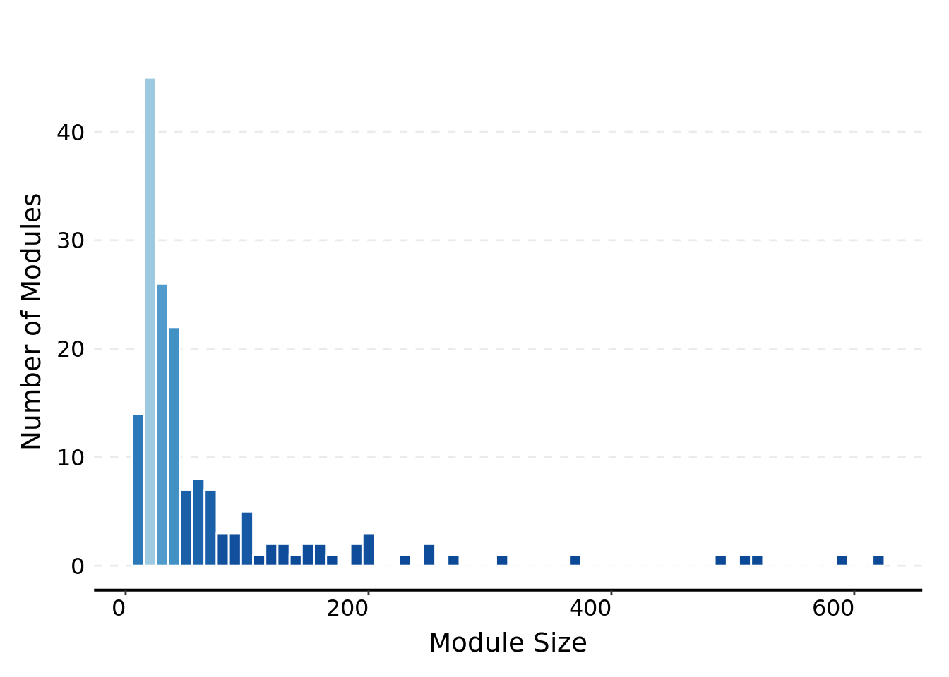
Look at the co-expression modules and module sizes
file_coexp_module <- "/project2/xuanyao/llw/DGN_no_filter_on_mappability/result/coexp.module.rds"
coexp_module <- readRDS(file_coexp_module)$moduleLabels


# modules and their sizes
df_module <- tibble("gene" = names(coexp_module),
                       "module" = coexp_module)
df_module_size <- df_module %>% group_by(module) %>% summarise(module_size = n())
There are 166 co-expression modules in total, consisting of 12,132 genes.
cat(
  'There are', max(df_module$module),
  'co-expression modules in total, consisting of',
  nrow(df_module), 'genes. \n\n'
)
## There are 166 co-expression modules in total, consisting of 12132 genes.The module sizes are distributed as below.
# histogram of number of modules v.s. module size
base_plt <- ggplot(df_module_size) +
  geom_histogram(aes(x = module_size, fill = after_stat(count)),
                 binwidth = 10,
                 color = "white") +
  scale_fill_gradientn(colors = RColorBrewer::brewer.pal(8, "Blues")[8:4],
                       na.value = "red") +
  labs(x = "Module Size", y = "Number of Modules")

base_plt +
  theme_classic() +
  theme(panel.grid.major.y = element_line(linetype = "dashed"),
        panel.background = element_rect(fill = "white"),

        legend.position = "none",
        legend.text = element_text(size = 10),
        legend.title = element_text(size = 10, face = "bold"),
        legend.background = element_rect(color = "black", linetype = "dashed"),
        legend.key.size= unit(0.5, "cm"),

        axis.line = element_line(colour="black", size = 0.7),
        axis.line.y = element_blank(),
        axis.ticks.y = element_blank(),

        plot.margin=unit(c(10,5,5,5),"mm"),
        axis.text.x = element_text(colour="black", hjust=1, vjust = 1, size = 12),
        axis.text.y = element_text(colour = "black", size = 12),
        axis.title.x = element_text(vjust = -0.2, size=14),
        axis.title.y = element_text(angle=90,vjust =2, size=14)
  )
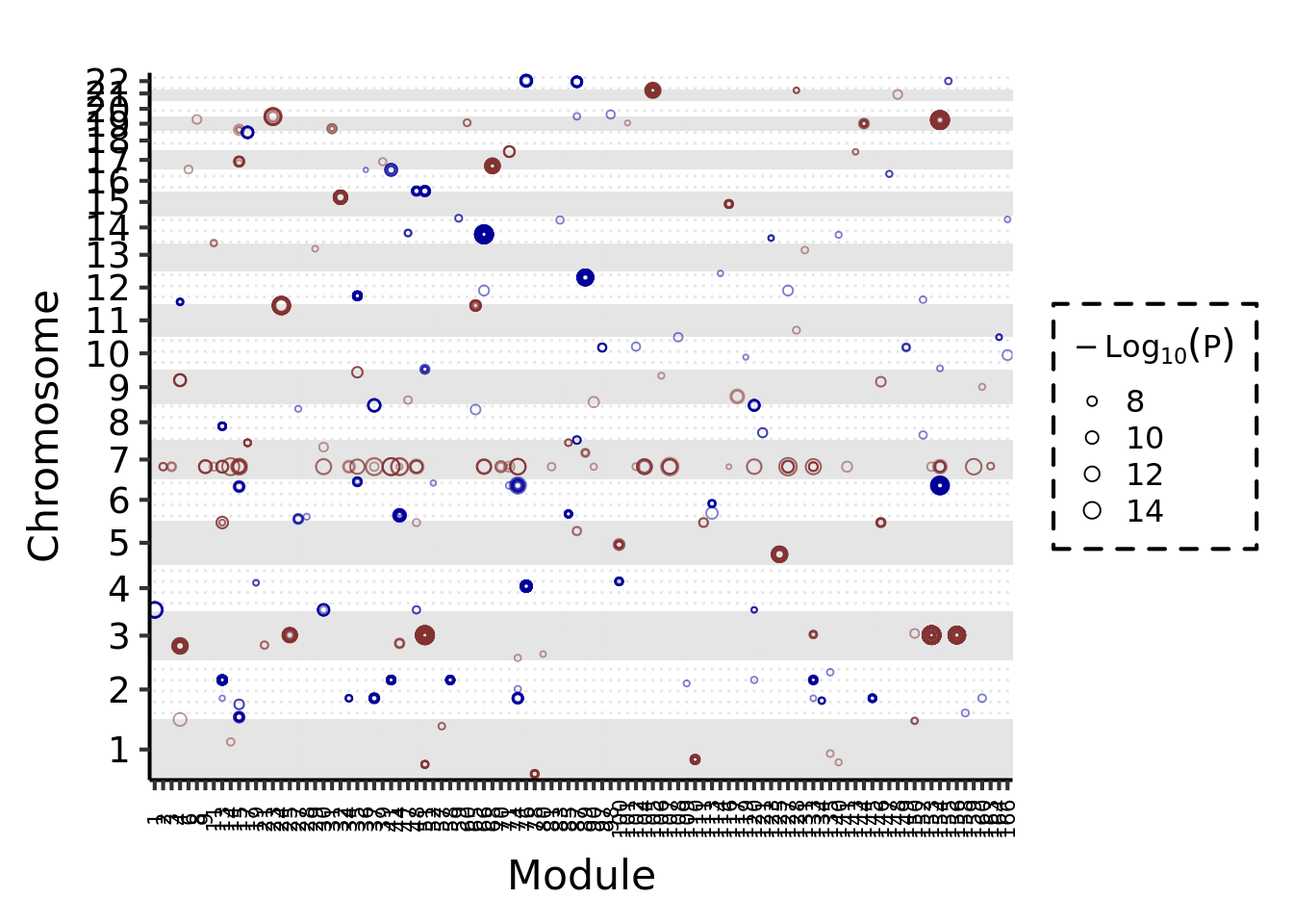
Trans signals and their corresponding trans target modules
Figure below: Signals of each module on chromosomes. Y-axis is chromosome position. X-axis shows module. Each point is a signal. Point size means -logP.
# I/O & paras -----
file_chr_pos <- '/scratch/midway2/liliw1/sig_module_chr/chromosome_location.rds'
file_qtl <- '/project2/xuanyao/llw/DGN_no_filter_on_mappability/FDR/signals.chr.module.perm10.fdr10.txt'


# read files -----
chr_pos <- readRDS(file_chr_pos)
qtl <- fread(file_qtl, header = FALSE, col.names = c("signal", "p", "q"))


# organize data -----
qtl <- qtl %>%
  separate(signal, c("module", "chr", "pos"), ":", remove = FALSE, convert = TRUE) %>%
  unite("SNP_ID", chr, pos, sep = ":", remove = FALSE) %>%
  separate(module, c(NA, "module"), sep = 'module', convert = TRUE)


# plot -logp for (cht pos, module) -----
plt_dat <- qtl %>%
  left_join(chr_pos, by = c("chr" = "CHR")) %>%
  mutate(def_pos = pos + tot)

base_plt <- ggplot(plt_dat, aes(y = def_pos, x = factor(module))) +
  geom_rect(
    aes(ymin = tot, ymax = xmax,
        xmin = -Inf, xmax = Inf,
        fill = factor(chr))
  ) +
  geom_vline(aes(xintercept = factor(module)),
             linetype = "dotted", color = "#e5e5e5") +
  geom_point(aes(size = -log10(p), color = factor(chr)),
             alpha = 0.5, shape = 1) +
  labs(x = "Module", y = "Chromosome", size = quote(-Log[10](P)))

base_plt +
  scale_y_continuous(
    limits = c(0, max(chr_pos$center)*2 - max(chr_pos$tot)),
    label = chr_pos$CHR,
    breaks = chr_pos$center,
    expand = c(0, 0)
  ) +
  scale_size(guide = guide_legend(override.aes = list(alpha = 1)), range = c(0.5, 3)) +
  scale_color_manual(values = rep(c("#843232", "#000099"), 22), guide = "none") +
  scale_fill_manual(values = rep(c("#e5e5e5", "#ffffff"), 22), guide = "none") +
  theme_my_pub() +
  theme(
    axis.text.x = element_text(angle = 90, size = 8)
  )
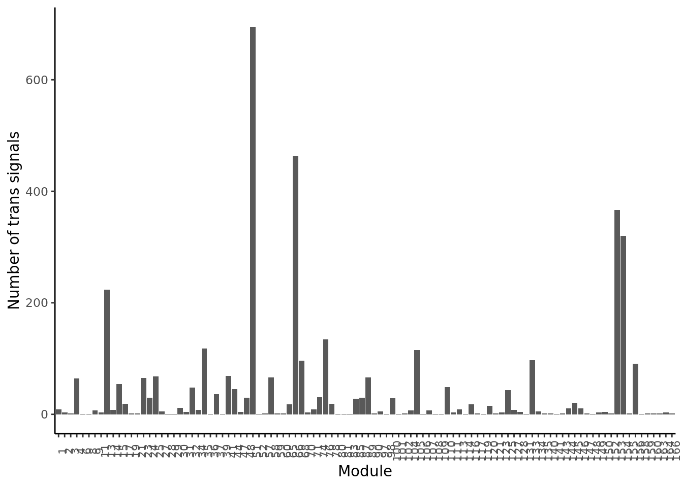
Distribution of trans signals on their corresponding target modules
ggplot(qtl) +
  geom_bar(aes(x = as.factor(module))) +
  labs(x = "Module", y = "Number of trans signals") +
  theme_classic() +
  theme(
    axis.text.x = element_text(angle = 90, size = 8)
  )
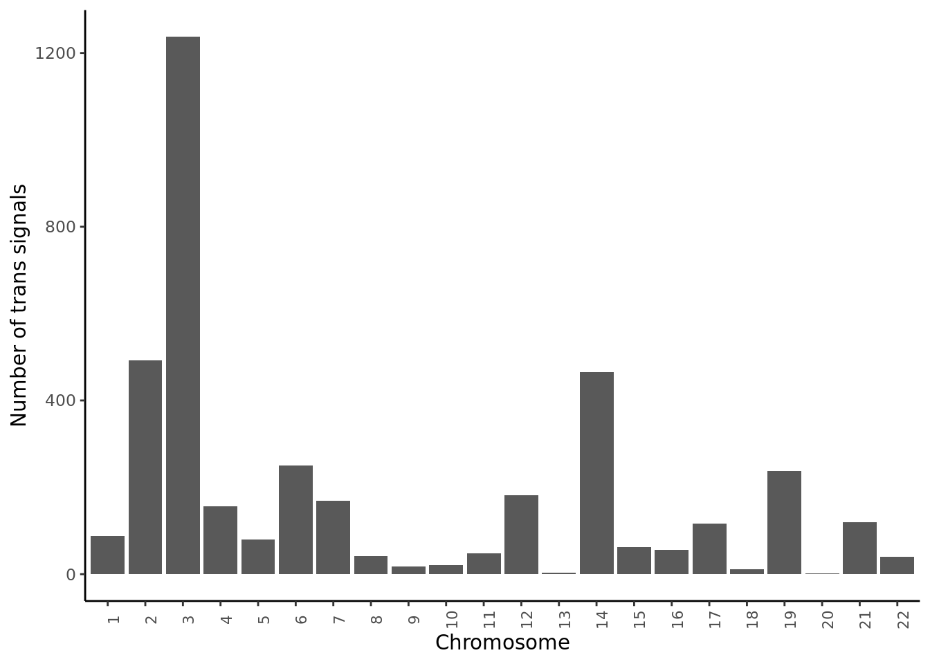
Distribution of trans signals on chromosomes
ggplot(qtl) +
  geom_bar(aes(x = as.factor(chr))) +
  labs(x = "Chromosome", y = "Number of trans signals") +
  theme_classic() +
  theme(
    axis.text.x = element_text(angle = 90, size = 8)
  )
Session info
sessionInfo()## R version 4.1.2 (2021-11-01)
## Platform: x86_64-conda-linux-gnu (64-bit)
## Running under: Ubuntu 20.04.3 LTS
##
## Matrix products: default
## BLAS/LAPACK: /scratch/midway2/liliw1/conda_env/rstudio-server/lib/libopenblasp-r0.3.18.so
##
## locale:
## [1] LC_CTYPE=en_US.UTF-8 LC_NUMERIC=C
## [3] LC_TIME=en_US.UTF-8 LC_COLLATE=en_US.UTF-8
## [5] LC_MONETARY=en_US.UTF-8 LC_MESSAGES=en_US.UTF-8
## [7] LC_PAPER=en_US.UTF-8 LC_NAME=C
## [9] LC_ADDRESS=C LC_TELEPHONE=C
## [11] LC_MEASUREMENT=en_US.UTF-8 LC_IDENTIFICATION=C
##
## attached base packages:
## [1] stats graphics grDevices utils datasets methods base
##
## other attached packages:
## [1] forcats_0.5.1 stringr_1.4.0 dplyr_1.0.7 purrr_0.3.4
## [5] readr_2.1.2 tidyr_1.2.0 tibble_3.1.7 ggplot2_3.3.6
## [9] tidyverse_1.3.1 data.table_1.14.2
##
## loaded via a namespace (and not attached):
## [1] tidyselect_1.1.1 xfun_0.29 bslib_0.3.1 haven_2.4.3
## [5] colorspace_2.0-3 vctrs_0.4.1 generics_0.1.2 htmltools_0.5.2
## [9] yaml_2.2.2 utf8_1.2.2 rlang_1.0.3 jquerylib_0.1.4
## [13] pillar_1.7.0 withr_2.5.0 glue_1.6.2 DBI_1.1.3
## [17] RColorBrewer_1.1-3 dbplyr_2.1.1 modelr_0.1.8 readxl_1.3.1
## [21] lifecycle_1.0.1 cellranger_1.1.0 munsell_0.5.0 gtable_0.3.0
## [25] rvest_1.0.2 evaluate_0.14 labeling_0.4.2 knitr_1.37
## [29] tzdb_0.2.0 fastmap_1.1.0 fansi_1.0.3 highr_0.9
## [33] Rcpp_1.0.8.3 broom_0.7.12 backports_1.4.1 scales_1.2.0
## [37] jsonlite_1.7.3 farver_2.1.1 fs_1.5.2 hms_1.1.1
## [41] digest_0.6.29 stringi_1.7.6 grid_4.1.2 cli_3.3.0
## [45] tools_4.1.2 magrittr_2.0.3 sass_0.4.0 crayon_1.5.1
## [49] pkgconfig_2.0.3 ellipsis_0.3.2 xml2_1.3.3 reprex_2.0.1
## [53] lubridate_1.8.0 assertthat_0.2.1 rmarkdown_2.11 httr_1.4.2
## [57] rstudioapi_0.13 R6_2.5.1 compiler_4.1.2